
Conditional formatting in Excel changes a cell’s colour, font or border when its value meets a rule. Select the cells, go to Home, then Conditional Formatting, and pick a built-in rule such as Greater Than or Duplicate Values. For anything more specific, choose New Rule and use a formula that returns TRUE for the cells you want to format.
The five kinds of rule
- Highlight Cells Rules: greater than, less than, between, equal to, text that contains, a date occurring and duplicate values.
- Top/Bottom Rules: top or bottom ten items or percent, and above or below average.
- Data Bars: a bar inside each cell whose length follows the value. Good for progress columns.
- Color Scales: a two or three colour gradient across a range, useful for spotting highs and lows in a grid.
- Icon Sets: arrows, flags or traffic lights by value band.
Microsoft’s own guide points out that the same rules work on a plain range, an Excel table and, in Excel for Windows, a PivotTable. Tables are the better home for most rules, because new rows pick up the formatting automatically.
How formula rules work
A formula rule is written for the top-left cell of the range you selected, and Excel adjusts it for every other cell, exactly as it would when you copy a formula. The rule formats a cell when the formula returns TRUE. That one idea explains almost every rule that “doesn’t work”:
- Select the range first, starting from the top-left cell, then write the formula for that cell.
- Put a dollar sign before the column letter (
$D2) to colour a whole row based on one column. - Put a dollar sign before the row number (
C$1) to colour a whole column based on a header row. - Leave both off when each cell should test itself.
Eight formulas worth keeping
Each assumes your data starts in row 2. Create them under Home, Conditional Formatting, New Rule, “Use a formula to determine which cells to format”.
- Overdue tasks (whole row):
=AND($D2<TODAY(), $E2<>"Done"), where D holds the due date and E the status. - Due in the next seven days:
=AND($D2>=TODAY(), $D2<=TODAY()+7). - Weekends in a date row:
=WEEKDAY(C$1, 2)>5. - Today’s column in a calendar or Gantt grid:
=C$1=TODAY(). - Every other row:
=MOD(ROW(), 2)=0. - Duplicates in one column, from the second occurrence on:
=COUNTIF($A$2:$A2, $A2)>1. - Blank required fields:
=AND($A2<>"", $C2="")flags a row that has a name but no amount. - Over budget:
=$F2>$E2, where E is the budget and F the actual.
Order, priority and Stop If True
When several rules apply to the same cell, Excel applies them in the order shown in Manage Rules, from the top. If two rules set the same property, such as the fill colour, the higher one wins; if they set different properties, both show. In Excel for Windows, ticking Stop If True on a rule prevents the rules below it from being checked for that cell, which is useful when “Done” should override “Overdue”.
Keep rules from multiplying
Copying and pasting cells, or inserting rows in the middle of a range, makes Excel split one rule into several with fragmented “Applies to” ranges. After a few weeks a sheet can carry dozens of near-identical rules and slow down noticeably. Three habits prevent it:
- Apply rules to whole table columns rather than to hand-picked ranges.
- Paste values only (Ctrl+Alt+V, then V) when moving data inside a formatted area.
- Every so often, open Manage Rules with “This Worksheet” selected, delete the duplicates and widen one rule’s range to cover the area.
Things that trip people up
- Cells with errors are skipped. Microsoft notes that formatting is not applied to a cell whose formula returns an error. Wrap the formula in IFERROR if those cells should be coloured too.
- Dates stored as text never match date rules. If a date aligns left, Excel is treating it as text.
- Colour is not a filter you can trust in shared files. Use the rule’s logic in a Status column if other people need to filter by it.
- Too many colours stop meaning anything. Two or three rules per sheet is plenty: one for a problem, one for a warning and perhaps one for done.
Google Sheets works the same way
In Google Sheets the menu is Format, then Conditional formatting, and the formula option is “Custom formula is”. The dollar sign logic is identical, so every formula above works there unchanged. Sheets also applies rules in list order, top first.
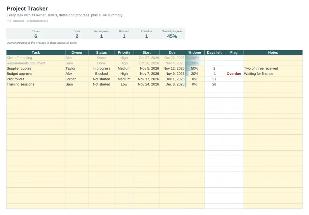
Our Excel templates use these rules for overdue flags, red months and progress bars, so you can see them working before you build your own.
Free Project Tracker Template for Excel
Status and priority dropdowns, an automatic Overdue or Blocked flag and progress bars per task, all driven by conditional formatting.
FAQ
Can conditional formatting be based on another sheet?
Yes. Current versions of Excel accept references to other sheets in a formula rule. In older versions, give the range a name and use the name instead.
How do I copy conditional formatting to another range?
Use Format Painter, or paste with Paste Special and choose Formats. Then check Manage Rules, because pasting can create a second copy of the rule instead of extending the first.
Does conditional formatting change the cell value?
No. It only changes how the cell looks. Formulas that read the cell see the same value as before.
Why does my rule colour the wrong rows?
The formula was written for a different starting cell than the one at the top of the selection, so every row tests the row above or below it. Reselect the range from its first cell and rewrite the rule for that cell.