
XLOOKUP searches one range for a value and returns the item in the same position from another range. Its three required arguments are what to find, where to look and what to return. It defaults to an exact match, can look left or right, can search from the bottom up and replaces both VLOOKUP and HLOOKUP.
The syntax
=XLOOKUP(lookup_value, lookup_array, return_array, [if_not_found], [match_mode], [search_mode])
- lookup_value: the thing you are looking for, such as a SKU or an employee ID.
- lookup_array: the single column or row to search.
- return_array: the column or row (or block of columns) to return from. It must be the same height as lookup_array.
- if_not_found: optional text or value to show instead of #N/A.
- match_mode: 0 exact (the default), -1 exact or next smaller, 1 exact or next larger, 2 wildcard.
- search_mode: 1 first to last (the default), -1 last to first, 2 and -2 binary search on sorted data.
XLOOKUP is available in Excel for Microsoft 365, Excel 2021 and 2024, Excel for the web and the mobile apps. Microsoft notes that it is not available in Excel 2016 or Excel 2019; a workbook that uses it will show errors there once the formulas recalculate. Google Sheets has its own XLOOKUP with the same arguments.
Why it replaced VLOOKUP
VLOOKUP asks for a column number, so inserting a column inside the table silently breaks every formula that points past it. It also defaults to an approximate match, which returns a wrong answer instead of an error when the value is missing, and it can only return columns to the right of the one it searches. XLOOKUP fixes all three: you point at the return column itself, the default is an exact match and the return range can sit anywhere.
Ten examples you will actually use
1. A basic exact match
Find the price of the SKU in F2, where SKUs are in A2:A200 and prices in D2:D200: =XLOOKUP(F2, A2:A200, D2:D200).
2. A friendly message instead of #N/A
=XLOOKUP(F2, A2:A200, D2:D200, "Not in list"). Use this on anything other people read; leave it out on working sheets where an error is a useful warning.
3. Looking to the left
If the SKU is in column D and the product name in column A, nothing changes: =XLOOKUP(F2, D2:D200, A2:A200). The return range does not have to be to the right.
4. Returning several columns at once
=XLOOKUP(F2, A2:A200, B2:D200) returns the name, supplier and price in three adjacent cells. The result spills to the right, so those cells must be empty.
5. The most recent entry
In a log where the same customer appears many times, set search_mode to -1 to get the last match instead of the first: =XLOOKUP(F2, B2:B500, E2:E500, , 0, -1). If the log is in date order, that is the latest entry.
6. Tax bands and price tiers
For a table of lower thresholds in ascending order, match_mode -1 returns the band the value falls in: =XLOOKUP(F2, A2:A8, B2:B8, , -1). An income of 52,000 against thresholds of 0, 11,000 and 44,725 returns the 44,725 row.
7. Wildcards
With match_mode 2, an asterisk stands for any run of characters: =XLOOKUP("*"&F2&"*", A2:A200, D2:D200, , 2) finds the first product whose name contains the text in F2.
8. Two criteria
Multiply two tests together and look for the 1 they produce where both are true: =XLOOKUP(1, (A2:A200=F2)*(B2:B200=G2), D2:D200). This finds the price for a given SKU at a given supplier without a helper column.
9. A two-way lookup
Nest one XLOOKUP inside another to pick a row and a column: =XLOOKUP(F2, A2:A13, XLOOKUP(G1, B1:M1, B2:M13)) returns the value for the month in F2 and the region in G1.
10. A case-sensitive match
XLOOKUP ignores case, so “abc” and “ABC” match. To tell them apart, look for TRUE in an EXACT test: =XLOOKUP(TRUE, EXACT(A2:A200, F2), D2:D200).
Common errors and how to fix them
- #N/A: no match. Usually a stray space or a number stored as text in one list and as a number in the other. TRIM the text, or convert both sides to the same type.
- #VALUE!: the lookup and return ranges have different sizes. A2:A200 against D2:D199 is enough to trigger it.
- #SPILL!: a multi-column result has nowhere to go. Clear the cells to the right or below.
- #NAME?: the file is open in a version without XLOOKUP, such as Excel 2016.
- Wrong band returned: with match_mode -1 or 1 the thresholds must be complete; with binary search modes (2 and -2) the data must also be sorted, or results are unreliable.
Make lookups easier to maintain
Turn the source list into an Excel table (Ctrl+T) and refer to its columns by name, as in =XLOOKUP(F2, Items[SKU], Items[Price]). The ranges then grow with the table, so new rows are found without editing a single formula. Lock fixed ranges with dollar signs before copying a formula down, or every copy will point one row lower than the last.
For more ready-to-use workbooks built on these functions, see our Excel templates guide.
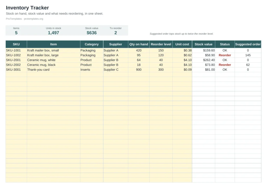
Free Inventory Tracker Template for Excel
An item list with SKU, supplier, quantity, reorder level and stock value, ready to feed lookups from an order sheet or a price list.
FAQ
Is XLOOKUP faster than INDEX and MATCH?
For everyday sheets the difference is too small to notice. On very large sorted lists, the binary search modes (2 and -2) are the fastest option either function offers.
Can XLOOKUP return a whole row?
Yes. Point return_array at a block of columns and the result spills across. This is handy for pulling a full record into a form or a summary.
What happens if the value appears twice?
XLOOKUP returns the first match from the top, or the last one if search_mode is -1. If you need every match, use FILTER instead.
Will my XLOOKUP formulas work for someone on Excel 2019?
No. Recent Excel versions store the last calculated result, so the values may show at first, but the formulas fail with #NAME? as soon as the sheet recalculates. Share a values-only copy or use INDEX and MATCH for that file.