
To make a Gantt chart in Excel, list your tasks with a start date and a duration in days, insert a stacked bar chart, hide the first series so only the duration bars remain, reverse the task order and set the date axis to start on your first day. The whole job takes about ten minutes.
What a Gantt chart shows, and why Excel needs a workaround
A Gantt chart puts each task on its own row and draws a horizontal bar from the day the task starts to the day it ends. Read down the rows and you see the order of the work; read across and you see what overlaps. The format goes back to Henry Gantt, an American engineer who developed it in the 1910s, and it has survived a century because it answers the two questions every project raises: what happens next, and is anything late.
Excel has no Gantt chart in its chart menu. Microsoft’s own support article says as much and builds the chart from a stacked bar chart instead. The trick is that a stacked bar chart draws two segments per row: the first (start date) pushes the second (duration) to the right place on the timeline. Make the first segment invisible and you have a Gantt chart.
Step 1: Set up the task table
Start with four columns in this order: Task, Start, Duration (days) and End. Only the first three feed the chart; End is there so you can check the dates at a glance.
- Task: a short name, ideally starting with a verb (“Draft brief”, “Review copy”).
- Start: a real Excel date, not text. If the cell aligns left by default, Excel is reading it as text.
- Duration: a number of calendar days.
- End: the formula
=B2+C2, copied down.
Keep the tasks in the order they happen. Excel will plot them in that order, which is what makes the finished chart readable.
Step 2: Insert a stacked bar chart
Select the Task and Start columns, including the headers. Go to Insert, open the bar chart menu and choose Stacked Bar (the 2-D version, with horizontal bars). Excel draws one bar per task, measured from zero, which looks wrong for now. That is expected.
Step 3: Add the duration series
Right-click the chart and choose Select Data. Click Add, name the series Duration and point Series values at the Duration cells (without the header). You now have two segments per task: a long one for the start date and a short one for the duration, stacked end to end.
Step 4: Hide the start-date bars
Click any of the start-date bars to select that whole series. In Format Data Series, set Fill to No fill and Border to No line. The bars vanish, and the duration bars float at the right point on the timeline. This is the step that turns a bar chart into a Gantt chart.
Step 5: Put the first task at the top
Excel plots the first row of data at the bottom of a bar chart. To fix it, select the vertical axis (the task names), open Format Axis and tick Categories in reverse order. Your first task now sits at the top, as people expect to read a plan.
Step 6: Fix the date axis
The horizontal axis usually starts at zero, which Excel reads as 1900, so your bars sit far to the right. Excel stores dates as serial numbers, so you need the number behind your first start date. Type the date in a spare cell, change its format to General and note the number (for example, 46000). In Format Axis, set the Minimum bound to that number. Set the Maximum bound to the number of your last end date, and the Major unit to 7 for weekly gridlines.
Step 7: Make it readable
- Set Gap Width on the duration series to around 40% so the bars are thick enough to read.
- Give the chart a plain title and delete the legend; with one visible series it adds nothing.
- Change the date format on the axis to something short, such as “d mmm”.
Step 8: Keep it updated
The chart is live: change a start date or a duration in the table and the bar moves. A simple routine keeps it trustworthy: update the table once a week, add a Status column (Not started, In progress, Done) and colour the bars by status if you want to see progress at a glance. When a task slips, change its start date rather than stretching its duration, so the chart shows what really happened.
Common problems and quick fixes
- All bars start at the same point: the Start cells are text. Re-enter them as dates or use DATEVALUE.
- Tasks appear in reverse order: you skipped Step 5.
- Bars are squashed to the right: the axis minimum is still zero. Redo Step 6.
- Weekends make bars look too long: durations here are calendar days. If you plan in working days, calculate the end date with WORKDAY and keep the chart duration as End minus Start.
When a template is the faster option
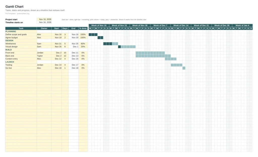
Building the chart once is a good way to understand it. For a real project, a template saves the setup and adds the parts you would otherwise build by hand, such as conditional formatting for today’s date, status colours and a progress column.
Free Gantt Chart Template for Excel
A ready-made Gantt chart with the task table, timeline and status colours already set up. Change the dates and the bars follow.
FAQ
Does Excel have a built-in Gantt chart?
No. Excel has no Gantt chart type. The usual method, the one Microsoft documents, is a stacked bar chart with the start-date series made invisible.
Can I show dependencies between tasks?
Not natively. You can add a Depends on column and calculate each start date from the end date of the task it depends on, so the bars move together when something slips.
How do I show today on the chart?
Add a scatter series with today’s date as the X value and draw it as a vertical line, or use conditional formatting in a grid-style Gantt chart built with cells instead of a chart.
Will it work in Google Sheets?
The same idea works in Google Sheets with a stacked bar chart, though the axis settings are in different menus. A cell-based Gantt chart with conditional formatting is often simpler there.